Recommendation System - Part II

Easy Way to build Recommendation System using Content-based Filtering—In Python–Part-2

In Part-1 we learned a lot of about Collaborative Filtering. In this article we will be taking a look at Content-based Filtering.

What is Content-based Filtering?

Content-based filtering is the one of the other technique that can be used to recommend items to the user. It does it so by recommending items to user based on the “content”, meaning items that the user may have either purchased or used or liked or disliked. Eg: Recommending Movie1 to ‘X ‘user based on the Movie2 and Movie3 that ‘X’ user has viewed or rated before.

Content-based Filtering Concepts

In part-1 we used Euclidean Distance Score to measure similairyt score but this time we are going to do so by using Pearson Corelation method. You can actually use former method to calculate score there’s nothing wrong with it. We are just changing method just to spice a things little bit.

Pearson Correlation Score

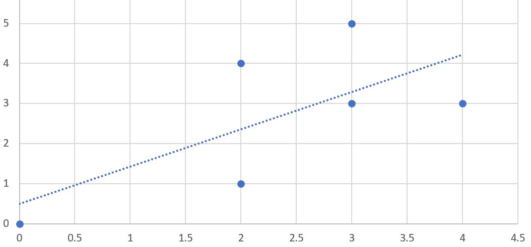
The correlation coefficient is a measure of how well two sets of data fit on a straight line. To visualize this method, you can plot the ratings of two of the critics on a chart, as shown in Figure 1. Movie1 was rated 3 by User1 and 5 by User2, so it is placed at (3,5) on the chart.

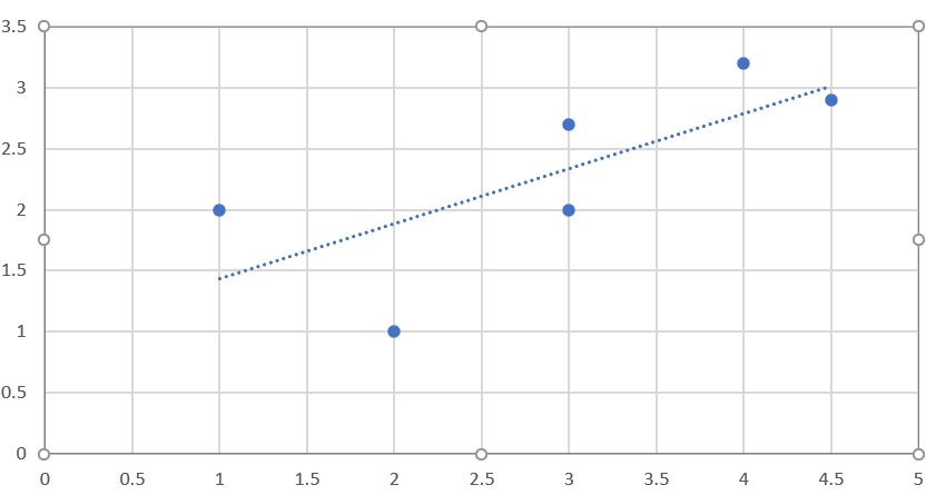
You can also see a straight line on the chart. This is called the best-fit line because it comes as close to all the items on the chart as possible. If the two critics had identical ratings for every movie, this line would be diagonal and would touch every item in the chart, giving a perfect correlation score of 1. In the case illustrated, the critics disagree on a few movies, so the correlation score is about 0.4. Figure 2-3 shows an example of a much higher correlation, one of about 0.75.

How to calculate the score for two users using pearson method?

Let X be the user1’s rated data and Y be the user2’s rated data then it looks somthing like this

Table-1. Pearson Co-relation Score

Here r gives the similarity score

Item comparison

In part-1 we compared the users and their similarity, we are going to do same but this time for item. Example: let’s say user1 has rated movie1 and movie2. In a dataset there are rating of movie3,movie4,.. so on. We are going to find how similar the movie1 is with other dataset movie2,movie4,.. and similary for movie2 also same. .

Create a file called contentfilter.py in your directory and add the following code in it.

def loadMovieLens(path='/data/movielens'):
    # Get movie titles
    movies={}
    for line in open(path+'/u.item'):
        (id,title)=line.split('|')[0:2] movies[id]=title
    # Load data
    prefs={}
        for line in open(path+'/u.data'):
            (user,movieid,rating,ts)=line.split('\t') prefs.setdefault(user,{})
            prefs[user][movies[movieid]]=float(rating)
    return prefs

This is the similar to previous code. It loads the movielens dataset and returns as prefs dictionary.

# Returns the Pearson correlation coefficient for p1 and p2
def sim_pearson(prefs,p1,p2): 
    # Get the list of mutually rated items
    si={}
    for item in prefs[p1]:
        if item in prefs[p2]: si[item]=1
    # Find the number of elements
    n=len(si)
    # if they are no ratings in common, return 0
    if n==0: return 0
    # Add up all the preferences
    
    sum1=sum([prefs[p1][it] for it in si])
    sum2=sum([prefs[p2][it] for it in si])
    # Sum up the squares
    sum1Sq=sum([pow(prefs[p1][it],2) for it in si])
    sum2Sq=sum([pow(prefs[p2][it],2) for it in si])
    # Sum up the products
    pSum=sum([prefs[p1][it]*prefs[p2][it] for it in si])
    # Calculate Pearson score
    num=pSum-(sum1*sum2/n)
    den=sqrt((sum1Sq-pow(sum1,2)/n)*(sum2Sq-pow(sum2,2)/n))
    if den==0: return 0
    r=num/den
    return r

Above function calculates the r which is a similarity score of the items. Now we have similarity score and dataset we are ready to make a recommendation but before that let’s add some code.

def transformPrefs(prefs):
    result={}
    for person in prefs:
        for item in prefs[person]:
            result.setdefault(item,{})
            # Flip item and person
            result[item][person]=prefs[person][item]
    return result

We have a dataset in the form of {‘user1’:{movie1:’4.5’,movie2:’3’}} with transformPrefs() function we are converting it to be item-centric rather than user-centric. Eg: {‘movie1’:{user1:’4.5’},’movie2’:{‘user1:’3’}} by transforming it now we can calculate similaity of items

def topMatches(prefs,person,n=5,similarity=sim_pearson):
    scores=[(similarity(prefs,person,other),other) for other in prefs if other!=person]
    # print(scores)
    # Sort the list so the highest scores appear at the top
    scores.sort()
    scores.reverse()
    return scores[0:n]

It’s the same function as before in part-1 which return highest matching item in reverse order

def calculateSimilarItems(prefs,n=10):
    # Create a dictionary of items showing which other items they
    # are most similar to.
    result={}
    # Invert the preference matrix to be item-centric
    # print(prefs)
    # print('----------------------------------')
    itemPrefs=transformPrefs(prefs)
    # print(itemPrefs)
    c=0
    for item in itemPrefs:
        # Status updates for large datasets
        c+=1
        if c%100==0: pass
        # Find the most similar items to this one
        scores=topMatches(itemPrefs,item,n=n,similarity=sim_distance)
        result[item]=scores
    return result

Now we calculate similarity for each items using calculateSimilarItems() function. The last part is getting recommendations

Content-based Recommendations Theory

Let’s look at how things have changed in more layman terms. We will create a table to make it more understandable. Table-2 shows the process of finding recommendation using Content-based Filtering approch. Unlike part-1 there was user involved in the recommendation and instead there is a grid of movies that a particular user ‘Bobby’ has rated. This is why we have created transformPrefs(prefs).

Table-2. Content-based recommendations for Bobby

Column movie and Rating show the movies that that Bobby has seen and rated personally. For every movie that Bobby haven’t seen,there’s a column that shows how similar it is to the movie that he has seen–for example the similarity score between superman and batman is 0.103. The column R.x is the muliplication of rating by similarity–4.0*0.103 = 0.412. And the predicated rating for Batman is 1.378/0.433 = 3.183

Content-based Recommendations Practical

def getRecommendedContent(prefs,itemMatch,user):
    userRatings=prefs[user]
    scores={}
    totalSim={}
    # Loop over items rated by this user
    for (item,rating) in userRatings.items( ):
        # Loop over items similar to this one
        for (similarity,item2) in itemMatch[item]:
            # Ignore if this user has already rated this item
            if item2 in userRatings: continue
            # Weighted sum of rating times similarity
            scores.setdefault(item2,0)
            scores[item2]+=similarity*rating
            # Sum of all the similarities
            totalSim.setdefault(item2,0)
            totalSim[item2]+=similarity
    # Divide each total score by total weighting to get an average
    rankings=[(score/totalSim[item],item) for item,score in scores.items( )]
    # Return the rankings from highest to lowest
    rankings.sort( )
    rankings.reverse( )
    return rankings

This is the python form of the Table-2 which the returns dictionary of recommended movie. now let’s load the dataset and start calling the function.

prefs=loadMovieLens()
items=calculateSimilarItems(prefs,n=50)
print(getRecommendedItems(prefs,items,'87')[0:30]) 

Here we are loading the movies and store it in prefs the we are calcualting similar items and storing it in items the finally getting recommentionf in last line

$ python3 contentfilter.py
[(5.0, "What's Eating Gilbert Grape (1993)"), (5.0, 'Vertigo (1958)'),
 (5.0, 'Usual Suspects, The (1995)'), (5.0, 'Toy Story (1995)'),...]

There you go we have created a Content-based filtering.

Conclusion

Content-based filtering is significantly faster than user-based when getting a list of recommendations for a large dataset, but it does have the additional overhead of maintaining the item similarity table. Also, there is a difference in accuracy that depends on how “sparse” the dataset is. Time and again we only need to calculate the similarity score of the items and then use it while making recommention. This is way it is useful in large dataset whose value rarely changes. User-based filtering is simpler to implement and doesn’t have the extra steps, so it is often more appropriate with smaller in-memory datasets that change very frequently